Chapter 6 Mortality plateaus

6.1 Outline

Mathematical background
Ken’s class
Presentation

6.2 Heterogeneity slows mortality improvement

Define $\rho(x,t)$ be the rate of mortality \[ \rho(x,t) = - {d \over dt} \log \bar\mu(x,t) \]

Extending our gamma result for 1 cohort to the surface, \[ \bar\mu(x,t) = \mu_0(x,t) \bar{S}_c(x,t)^{\sigma^2} \]

We take the log and the time-derivative of hazards give Vaupel and Missov (2014) (Eq. 39*) \[ \rho(x,t) = \rho_0(x,t) - \sigma^2 {d \over dt} \log \bar{S}_c(x,t)^{\sigma^2} \]

Note: this formula should be correct. Vaupel and Missov (2014) contains a mistake: an extra minus sign in the definition of $\bar{S}_c(x,t)$.

We take the log and the time-derivative of hazards give Vaupel and Missov (2014) (Eq. 39*)

\[ \rho(x,t) = \rho_0(x,t) - \sigma^2 {d \over dt} \log \bar{S}_c(x,t) \]

So individual risks from one cohort to the next are going down faster it seems. Intuition?

Reversing perspective,

\[ \rho_0(x,t) = \rho(x,t) + \sigma^2 {d \over dt} \log \bar{S}_c(x,t) \]

6.2.1 An example

Assume $\sigma^2 = .2$.

library(data.table)
  sigma.sq = .2
  dt <- fread("/hdir/0/fmenares/Book/bookdown-master/data/ITA.bltcoh_1x1.txt", na.string = ".")
  mx.80.c1880 <- dt[Year == 1880 & Age == "80"]$mx
  mx.80.c1900 <- dt[Year == 1900 & Age == "80"]$mx
  (rho.bar.80 <- -log(mx.80.c1900/mx.80.c1880)/20) ## about 0.8%

## [1] 0.008729961

  Sx.80.c1880 <- dt[Year == 1880 & Age == "80"]$lx
  Sx.80.c1900 <- dt[Year == 1900 & Age == "80"]$lx
  (d.log.Sx <- log(Sx.80.c1900/Sx.80.c1880)/20)

## [1] 0.02177952

  (rho.0.80 = rho.bar.80 + sigma.sq * d.log.Sx) ##  about 1.3%

## [1] 0.01308586

So individual-level mortality progress is nearly 50% faster (1.3% vs. 0.9%) than it appears!

6.3 Conclusions

Gamma frailty gives simple expressions for population survival, hazard, and average frailty.
Gamma frailty gives a plateau.
Gamma frailty gives us a predicted rate of convergence and cross-over with age.
All of this means it is a useful null model.
Takes us away from “it could be selection” to “what if it were selection”.

6.4 Hazards and Plateaus by Professor Ken Wachter

6.4.1 Outline

Extremes of Longevity in Humans and Other Species
Gamma-Gompertz Fixed Frailty Hazards
Less Restrictive Frailty Models
Mutation Accumulation, Gompertz Hazards with Plateaus

Note: we thank Professor Kenneth Wachter for letting us use the presentation and code from his class on Hazards and Plateaus on February 20, 2020 at Demography UC Berkeley.

6.4.2 Extremes of Longevity in Humans and Other Species

Estimated plateau for cohort of Italian women from 1904. Source: @barbi2018

Figure 6.1: Estimated plateau for cohort of Italian women from 1904. Source: Barbi et al. (2018)

What is the importance of plateaus?

They encourage optimism that future progress against old-age mortality is feasible. Our bodies are not facing an endlessly mounting set of things going wrong.
They point to commonalities with the life-course demography of other species. The shared genetic heritage of advanced organisms is permissive.

For instance, we can compare human hazard to that of other species:

Figure 6.2: Hazards across selected species. Source: Horiuchi (2003)

6.4.3 Gamma-Gompertz Fixed Frailty Hazards

The Gamma-Gompertz model of Vaupel, Manton, and Stallard (1979) is familiar from this course and Chapter 8 of Essential Demographic Methods (Wachter 2014).
Gamma Gompertz models are one way of generating plateaus for population hazards out of increasing individual hazards.
We fit parameters to the data in Barbi et al. (2018) and look for a predicted plateau, starting from age 60 onwards.
We need formulas for the individual hazard $h_x$ , for the individual cumulative hazard $H_x$, and for the aggregate population hazard $\mu_x$ implied by Gamma-distributed frailty with shape parameter $k$ and rate parameter $\theta = k$.
Does the prediction show a plateau?
Does the level of the plateau fit plateau observed in the Italian cohorts over age 105?

To answer these questions, we create the process below to calculate the aggregate population hazard function predicted from Gompertz hazards for individuals combined with a Gamma distribution for fixed proportional frailty, using parameters matched to the Italian cohort data for Barbi et al. (2018).

    # Parameters for Gompertz and Gamma 
    beta     <-  0.088            #  Gompertz slope parameter,  Barbi et al.
    alpha60  <-  0.01340671       #  Gompertz intercept parameter at age 60 
    asymp    <-  0.620            #  Observed asymptote, for comparisons in plots
    khat     <-  7.045455         #  Gamma shape parameter, to fit plateau 
    theta    <-  1/khat           #  Gamma rate parameter, for unit mean at 60
    # Age range, starting to observe cohorts at age 60, reaching up to 130 
    xxx      <-  c(0:200)          #  set of values of x, years past 60
    age      <-  60  +  xxx       #  age  

    # Hazards: 
    ###  Gompertz formula to calculate individual hazards hx at x:
    hx       <-  alpha60 *exp(beta*xxx) ##also noted as mu_0(x) in course material
    ###  Individual cumulative hazard  Hx formula
    Hx       <-  cumsum(hx) ## another way of getting it is  (a/b)(exp(bx)-1)
    ###  Aggregate population hazard mu_x with Gamma frailty:
    mux       <-  hx *khat/ (khat + Hx)

    #Plot:
    plot(age, log(hx), type= "l", col="blue", xlim = c(60,130), ylim =c(min(log(hx)),4),
         xlab= "Ages for estimated Gompertz", ylab="Log hazard") #individual hazard
    lines(age, log(mux), col="red")           #predicted population hazard
    segments(x0 = 104, x1 =117, y0 = log(asymp) ) #estimated plateau from Barbi et al.
    legend("topleft", legend=c(expression("Individual hazard, h"[x]), 
                               "Predicted population hazard, "~ mu [x],
                               "Plateau estimate Barbi et al. (2018)"),
       col=c( "blue","red", "black"), lty=rep(1,3))

Figure 6.3: Hazards and plateau with Gamma frailty

Note that the x-axis shows the ages for the estimated Gompertz, that is for a population of ages 60 and above.
$\mu_x$ appears to reach its own plateau due to the chosen parameters from the Gamma-Gompertz model.
In this case, we get a plateau further along than in the italian case of Barbi et al. (2018).
Gamma gompertz models are good at fitting plateaus mathematically but may not be aplicable with the data.

6.4.3.1 How does Gamma Gompertz Make a Plateau?

Try alternative values for $k$ and for $\beta$. Guess a formula for the level of the plateau.

beta_vals <- c(0.001, 0.1, beta, 0.5,1,10)
k_vals <- c(0.1, 1, 3, khat,10)

plateau_beta_nolegend <- function(beta_vals, k_vals){
hx       <-  alpha60 *exp(beta_vals*xxx) ##also noted as mu_0(x) in course material
Hx       <-  cumsum(hx) ## another way of getting it is  (a/b)(exp(bx)-1)
mux      <-  hx *k_vals/ (k_vals + Hx)
    
    #Plot:
    plot(age, log(hx), type= "l", col="blue", xlim = c(60,130), ylim =c(min(log(hx)),4),
         xlab= "Ages for estimated Gompertz", ylab="Log hazard",
         main=bquote(beta == .(beta_vals))) #individual hazard
    lines(age, log(mux), col="red")           #predicted population hazard
    segments(x0 = 104, x1 =117, y0 = log(asymp) ) #estimated plateau from Barbi et al.
}
plateau_beta_legend <- function(beta_vals, k_vals){
hx       <-  alpha60 *exp(beta_vals*xxx) ##also noted as mu_0(x) in course material
Hx       <-  cumsum(hx) ## another way of getting it is  (a/b)(exp(bx)-1)
mux      <-  hx *k_vals/ (k_vals + Hx)
    
    #Plot:
    plot(age, log(hx), type= "l", col="blue", xlim = c(60,130), ylim =c(min(log(hx)),4),
         xlab= "Ages for estimated Gompertz", ylab="Log hazard",
         main=bquote(beta == .(beta_vals))) #individual hazard
    lines(age, log(mux), col="red")           #predicted population hazard
    segments(x0 = 104, x1 =117, y0 = log(asymp) ) #estimated plateau from Barbi et al.
           legend("bottomright", legend=c(expression("Individual hazard, h"[x]), 
                               "Predicted population hazard, "~ mu [x],
                               "Plateau estimate Barbi et al. (2018)"),
                  col=c( "blue","red", "black"), lty=rep(1,3), cex=0.7) 

}


plateau_k_nolegend <- function(beta_vals, k_vals){
hx       <-  alpha60 *exp(beta_vals*xxx) ##also noted as mu_0(x) in course material
Hx       <-  cumsum(hx) ## another way of getting it is  (a/b)(exp(bx)-1)
mux      <-  hx *k_vals/ (k_vals + Hx)
    
    #Plot:
    plot(age, log(hx), type= "l", col="blue", xlim = c(60,130), ylim =c(min(log(hx)),4),
         xlab= "Ages for estimated Gompertz", ylab="Log hazard",
         main=bquote(k == .(k_vals))) #individual hazard
    lines(age, log(mux), col="red")           #predicted population hazard
    segments(x0 = 104, x1 =117, y0 = log(asymp) ) #estimated plateau from Barbi et al.
}
plateau_k_legend <- function(beta_vals, k_vals){
hx       <-  alpha60 *exp(beta_vals*xxx) ##also noted as mu_0(x) in course material
Hx       <-  cumsum(hx) ## another way of getting it is  (a/b)(exp(bx)-1)
mux      <-  hx *k_vals/ (k_vals + Hx)
    
    #Plot:
    plot(age, log(hx), type= "l", col="blue", xlim = c(60,130), ylim =c(min(log(hx)),4),
         xlab= "Ages for estimated Gompertz", ylab="Log hazard",
         main=bquote(k == .(k_vals))) #individual hazard
    lines(age, log(mux), col="red")           #predicted population hazard
    segments(x0 = 104, x1 =117, y0 = log(asymp) ) #estimated plateau from Barbi et al.
           legend("topleft", legend=c(expression("Individual hazard, h"[x]), 
                               "Predicted population hazard, "~ mu [x],
                               "Plateau estimate Barbi et al. (2018)"),
                  col=c( "blue","red", "black"), lty=rep(1,3), cex=0.7) 

}

Here, we change the values of $\beta$ while fixing the $k$ shape factor of the Gamma frailty distribution.
As $\beta$ increases, the individual and population hazards rise (or shift upwards).
For comparison, the third panel contains the $\beta=0.088$ and $k=7.045455$ values used in the previous excercise.

par(mfrow=c(2,3))
plateau_beta_nolegend(beta_vals[1],khat)
plateau_beta_nolegend(beta_vals[2],khat)
plateau_beta_nolegend(beta_vals[3],khat)
plateau_beta_nolegend(beta_vals[4],khat)
plateau_beta_legend(beta_vals[5],khat)

Figure 6.4: Changing values of beta in Gompertz hazards

The following graphs fix $\beta=0.088$ but use different values of $k$.
Contrary to what happens when $\beta$ varies, when the shape parameter of the Gamma frailty distribution changes, only the population hazards appear to change.
Population hazards expand upwards with increases in $k$. The fourth panel uses the baseline values for $\beta=0.088$ and $k=7.045455$.

par(mfrow=c(2,3))
plateau_k_nolegend(beta,k_vals[1] )
plateau_k_nolegend(beta,k_vals[2] )
plateau_k_nolegend(beta,k_vals[3] )
plateau_k_nolegend(beta,k_vals[4] )
plateau_k_legend(beta,k_vals[5] )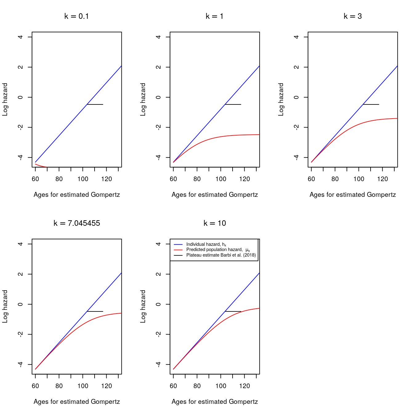

Figure 6.5: Changing values of k (Gamma shape parameter)

This formula can be proved by showing that $h_{x}/H_{x}$ goes to $\beta$ in a Gompertz model and plugging into the formula for Gamma Gompertz aggregate hazards. (Note for Josh: I don’t think Ken really explained this in class and I’m confused on how to answer this.)
What happens to the mean frailty of survivors as $x$ increases? What has to balance what in order for a plateau to appear?
- First, the mean frailty among survivors is the ratio of $\mu_x$ to $h_x$. In other words, the mean frailty among the people that remain is the population hazard divided by the individual hazard.
- The mean frailty falls across ages, such that around 105 years, the mean frailty is about 0.5. It continues decreasing until it reaches a plateau of about 0.1 starting from age 130 onwards. Survivors past 130 have a low mean frailty but at a higher hazard, as seen by the plateau from previous graph.
- The plateau comes from the people that are low frailty but that die. This loss balances out the increase that everyone is experiencing. Selection is balancing senescence.

plot( age, mux/hx, xlim = c(60, 200), type = "l"  , xlab = "", ylab = "Mean Frailty" )
abline( h = 0.5,  lty = 3     )                     # vertical age 105   
abline( h = 0.1,  lty = 3     )                     # vertical age 105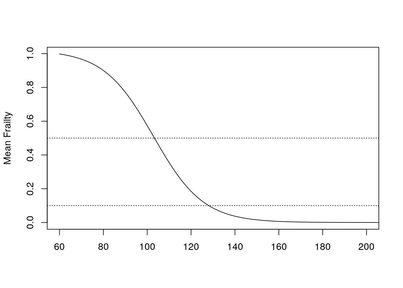

Figure 6.6: Mean frailty

6.4.3.2 Troubles with Gamma Gompertz:

Poor fits to observed cohort plateaus.
Unrealistic mortality rates at younger ages for those who do survive out onto the plateau. (The frailty distribution reaches down to zero frailty).
Individual centenarians still experience exponentially increasing hazards under the model.
Why should frailty remain fixed across life?
The model assumes rather than explains an underlying Gompertz.
There is no full genetic or evolutionary story.

6.4.3.3 Mathematics of Frailty as a Gamma Random Variable:

Probability density: $\left(\frac{\theta^{k}}{\Gamma(k)}\right)z^{k-1}e^{-\theta z}$
Mean: $\frac{k}{\theta}$
Variance: $\frac{k}{\theta^2}$
$\mathbb{E}e^{-ZH}= \left(\frac{\theta}{\theta H}\right)^{k}$
Exponential and Gamma Random Variables:
- When U has a uniform distribution on $[0, 1]$, then $Y = −log(U)/\theta$ has an exponential probability distribution on $(0,\infty)$ with mean $1/\theta$ and variance $1/\theta^2$.
- The sum of $k$ independent exponential random variables with the same mean $1/\theta$ has a gamma probability distribution with shape $k$, scale $\theta$, rate $1/\theta$, mean $k/\theta$ and variance $k/(\theta^2)$.
- With an exponential variable Y, we have $\mathbb{E}e^{-YH}=\int e^{-yH}p(y)dy= \frac{\theta}{\theta+H}$.
- Because expectation values of independent random variables multiply, with a gamma variable $Z = Y_1 + Y_2 + · · ·Y_k$, we have $\mathbb{E}e^{-ZH}= \left(\frac{\theta}{\theta+H}\right)^k$.

6.4.3.4 Vaupel, Manton, and Stallard (1979)

Lifelong Fixed Frailty Z.
The Gamma distribution has $\mathbb{E}e^{-ZH}= \left(\frac{\theta}{\theta+H}\right)^k$
For starting mean frailty equal to 1, we have $k = \theta$.
The aggregate population hazard is minus the slope of the logarithm of survivorship: $\mu_x = -\frac{d}{dx}\left(k log(\theta)- k log(\theta+H_x)\right)= \left(\frac{k}{\theta+H_x}\right)h_x$
For the Gamma Gompertz, we insert Gompertz individual hazards $h_x$ and individual cumulative hazards $H_x$ into the formula.

6.4.4 Less Restrictive Frailty Models

The key property of the Gamma Gompertz model is a frailty distribution that extends all the way down to zero frailty.
With any initial frailty distribution that extends down to zero and looks like a Gamma near zero, the frailty distribution among survivors comes to look like a Gamma.
If you do assume a Gamma distribution for frailty, then a plateau in the aggregate population hazard function entails an individual hazard function tending toward a Gompertz.
However:
- Frailties near zero are unrealistic.
- With frailties bounded away from zero, plateaus in aggregate hazards require plateaus in individual hazards
- Plateaus in individual hazards can arise naturally, for instance from genetic models.
Consider a “semi-circle” frailty whose probability density function is, for instance, $p(z) = (6)(z − 0.7)(1.3 − z)$ on $[0.7, 1.3]$, zero else.
If the individual hazard were Gompertz, would there be a plateau?
Suppose the individual hazard were given by $\frac{x}{(1 + x)}$.
- Would there be a plateau in the individual hazard? If so, at what level?
- Would there be a plateau in the aggregate population hazard? If so, at what level?
We ask what genetic processes might shape individual hazards into having stretches that look Gompertz and old-age forms looking like plateaus.

6.4.5 Mutation Accumulation, Gompertz Hazards with Plateaus

We turn to alternative models with plateaus in individual hazards, not just in aggregate population hazards.
The genetic evolutionary theory of “mutation accumulation” suggests one story to account both for Gompertzian increases over a stretch of adult ages and for plateaus beyond them.
We each inherit genetic variants or “alleles” in our DNA originating in mutations thousands of generations in the past.
Picture, say, the time of the cave painters, 40,000 B.C., when people died in their 30s and 40s and 50s rather than their 70s, 80s, and 90s, losing some of their chance to bear and raise offspring.

6.4.5.1 Mutation-Selection Equilibrium

Go back to basic stable (stationary) population theory. Write $\rho(a)$ for the size of the group of individuals (e.g. women) who carry a certain mutant allele indexed by the letter $a$.
The NRR for members of the group is assumed to be $1 − S(a)$ for some small “selective cost” $S(a)$ due to effects of the “deleterious” allele.
In the next generation, there are $\rho(a)(1 − S(a))$ daughters.
There are also $\nu(a)$ new arrivals due to new mutations.
The group keeps growing until it reaches equilibrium, when losses are balanced by new arrivals, and $\rho(a) = \rho(a)(1 − S(a)) + \nu(a)$.
Then, $\rho(a)$ as a function of $S(a)$ is: $\rho(a)= \frac{\nu(a)}{S(a)}$

6.4.5.2 Deleterious Alleles with Age-Specific Effects

In our setting, many deaths come from external threats regardless of age, a background level of “extrinsic mortality” with constant hazard $\lambda$.
To keep the story as simple as possible, picture a mutant allele that has a small bad effect on survival only at an “age of onset” $a$. It raises the hazard of the individual who carries it by an amount $\delta$ in the age interval $a$ to $a + 1$.
Picture a constant level of fertility from age 20 onward, set to make the NRR equal to 1 for women who carry no mutant alleles.
Take, for example, $\lambda = 0.080$, $\delta= 0.002$, and $\nu(a) = 0.020/50$ for any $a \geq 20$. For each separate choice of age of onset $a$, find and plot the equilibrium size $\rho(a)$ as a function of $a$.
- Here, we explore a genetic process which can generate a plateau in individual hazard functions. In particular, this is the case where a harmful mutant allele increases the hazard function of those that carry such allele with onset only in a single age interval.

# Parameters
lambda   <-   0.080           #  background extrinsic hazard 
delta    <-   0.002           #  increment to hazard from mutant allele
epsilon  <-   0.0005          #  fixed cost 
nu       <-   0.200/50        #  mutation rate per site per generation

# Range of ages  
xxx      <-  c(0:50)          #  set of values of x, years past 20, up to 70
age      <-  20  +  xxx       #  age  

# Fertility level that makes baseline NRR equal to 1.
lx       <-  exp(-lambda*xxx) #  survivorship under background hazard 
fert     <-  1/sum(lx) #total fertility or constant level of fertility

# Loop over choices of an age interval a at which the mutant allele affects the hazard.

bigrho   <-  NULL             #  vector for holding values of rho  

for  ( a in seq(xxx))      { 
  
  hxa    <- lambda + 0*xxx + 0*epsilon        #  baseline hazard (no fixed cost)  
  hxa[a] <- hxa[a]  + delta                   #  add hazard increment in age interval a 
  
  Hxa   <- c(0, cumsum(hxa))[seq(hxa)]
  lxa   <- exp(-Hxa) 

  Sa    <- 1 - sum( fert*lxa)   # S(a): Selective cost
  rho   <- nu/Sa                # Rho(a)
  
  bigrho <- c(bigrho, rho)    
}

$\rho(a)$ increases exponentially, this comes from the exponential survival. This graph tells us, the number of people that survive when the mutation is triggered at a given age. So at age 70, about 1400 people survive but if the mutation hit at age 20, nobody would survive.

par(mfrow=c(1,2))
plot(  age,  bigrho, ylab=expression(~rho(a)))
plot(  age,  log(bigrho), ylab =expression("log" ~rho(a))  )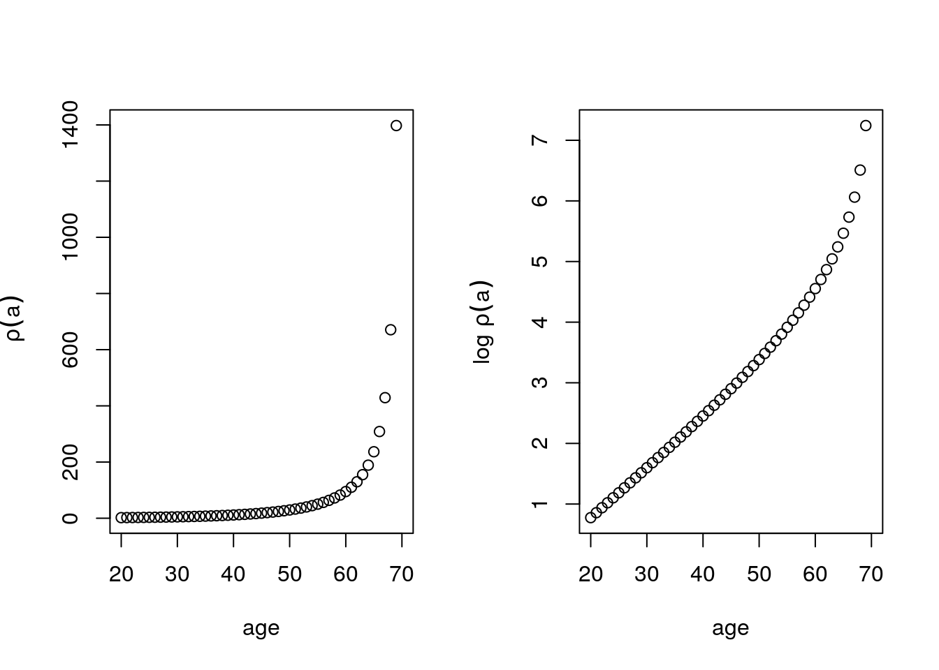

$$\rho(a)$ as a function of age$

Figure 6.7: $\rho(a)$ as a function of age

6.4.5.3 Allele Counts and Individual Hazards

Suppose that the alleles carried by an individual are a random sample of the alleles present in the population, so that $\rho(a)$ can be reinterpreted as the mean number of alleles of type $a$.
Then the hazard for an individual at age $a$ will look on average like the curve $\lambda + \rho(a) \times \delta$.
Does this curve resemble a Gompertz hazard? What about a Makeham hazard, that is, a Gompertz hazard plus a constant?
- This hazard looks like a Makeham hazard (Gompertz plus a constant).

hxx  <-  lambda +  bigrho*delta

plot ( age, hxx,  ylim = c(0,0.500) , ylab= "hazard")

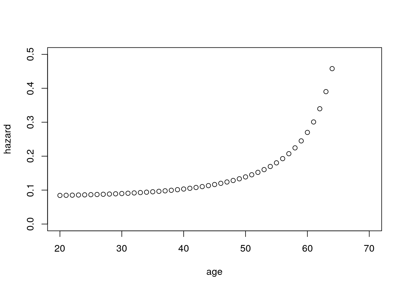
Figure 6.8: Hazard after exposure to allele

The background intrinsic mortality $\lambda$ comes from the environment, not from the DNA. What might happen to $\lambda$ as we move from the time of the cave painters to the time of the moon landings?

6.4.5.4 Plateaus in Allele Counts

Suppose, now, that each mutant allele raises the hazard by another small amount $\epsilon= 0.0005$ at all ages beyond 20, along with its special effect on raising the hazard by $\delta$ at age $a$.
Find and plot the size $\rho(a)$ of the carriers of a at equilibrium under this new form of action.
Is there an appearance of a plateau at high ages?
Is it plausible to expect some fixed cost along with an age-specific effect from mildly deleterious mutant alleles?
- Here is the case were a deleterious mutant allele imposes a fixed cost of size $\epsilon$ as well as adding an increment of size $\delta$ to the hazard in age interval $a$.
- There appears to be a plateau on the survivors after the onset of the mutation at age $a$ when we add a fixed cost to the mutation, even if it is happening late in the reproductive cycle.

#Loop over choices of an age interval a at which the mutant allele affects the hazard with fixed cost

bigrho2   <-  NULL             #  vector for holding values of rho  
for  ( a in seq(xxx))      {
  
  hxa    <- lambda + 0*xxx + epsilon        #  baseline hazard plus fixed cost epsilon
  hxa[a] <- hxa[a]  + delta                   #  add hazard increment in age interval a 
  
  Hxa   <- c(0, cumsum(hxa))[seq(hxa)]
  lxa   <- exp(-Hxa) 
  
  Sa    <- 1 - sum( fert*lxa)       #   Selective cost including allele at age a 
  rho   <- nu/Sa                    #   Equilibrium count of mutation a 
  
  bigrho2 <- c(bigrho2, rho)
}

par(mfrow=c(1,2))
plot(  age,  bigrho2, ylab=expression(~rho(a)))
plot(  age,  log(bigrho2), ylab =expression("log"~rho(a))  )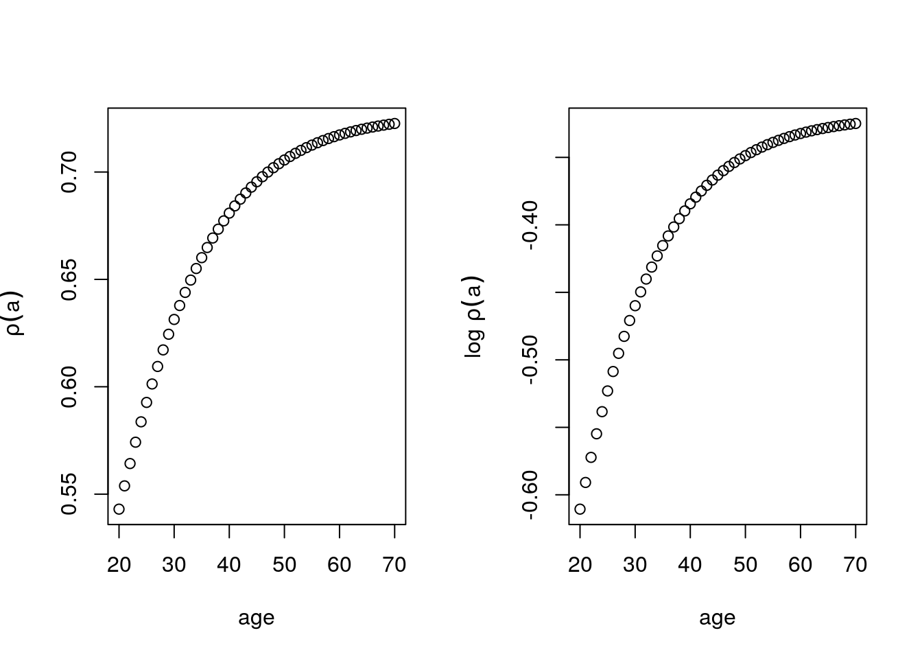

$$\rho(a)$ as a function of age$

Figure 6.9: $\rho(a)$ as a function of age

6.4.5.5 Questions for Further Study

What about the effect of each allele on the selective cost of all the other alleles?
Looking across species, under this account would we expect some relationship between the level of extrinsic background mortality and the steepness of the slope of a Gompertz increase in mortality with age?
In our calculation we let mortality over the age of 50 continue to reduce the “NRR”. Why might survival beyond ages of childbearing have an effect on generational replacement?
We carry in our DNA a load of mutant alleles shaped by natural selection over hundreds and thousands of generations. Why might it be that effects of those alleles that were once lethal in mid-adult life could now be influencing rates of mortality late in life for us?

6.5 Key points

Plateaus are significant information for demographers who try to predict future progress against old-age mortality. Gompertz discouragement – Plateau encouragement
Gamma-Gompertz models offer one explanation for plateaus, but no explanation for Gompertz acceleration, which is simply assumed. -In frailty models, plateaus come out of the specialness of survivors. The mathematics treats mixtures of survivorship.
Evolutionary genetic models aim to explain both Gompertz acceleration and old-age plateaus.
In the mutation-accumulation story, plateaus are present in the hazard functions of individuals, shaped by inherited genetic load.
In demography, survivorship is ALWAYS an exponential function of cumulative hazards.
In genetic stories, this exponential is the source of the exponential in the Gompertz formula.
The study of hazards at extreme age may inform our understanding of hazards at younger ages.

References

Barbi, Elisabetta, Francesco Lagona, Marco Marsili, James W Vaupel, and Kenneth W Wachter. 2018. “The Plateau of Human Mortality: Demography of Longevity Pioneers.” Science 360 (6396): 1459–61.

Horiuchi, Shiro. 2003. “Interspecies Differences in the Life Span Distribution: Humans Versus Invertebrates.” Population and Development Review 29: 127–51.

Vaupel, James W, Kenneth G Manton, and Eric Stallard. 1979. “The Impact of Heterogeneity in Individual Frailty on the Dynamics of Mortality.” Demography 16 (3): 439–54.

Vaupel, James W, and Trifon I Missov. 2014. “Unobserved Population Heterogeneity: A Review of Formal Relationships.” Demographic Research 31: 659–86. https://www.demographic-research.org/Volumes/Vol31/22/.

Wachter, Kenneth W. 2014. Essential Demographic Methods. Harvard University Press.