Chapter 5 Convergence and cross-overs
5.1 Outline
- Concepts
- Student Presentation
Additional resources:
5.2 What happens to mortality disparities at older ages?
- Cumulative disadvantage
- Age as a leveler
- Individual adaptation/plasticity, gov support, separation from unequal structures like labor market
- Bad data / measurement
- Unreliable ages, institutionalization changes sample, etc.
- Nothing
- It’s all selection (“frailty”), pop hazards but individual hazards would have remained “parallel”.
Our goal is to examine this last “null hypothesis”. What can frailty explain, and what can’t it
5.2.1 A possible null-model
2 groups, each with internal gamma-frailty
proportional baseline hazards
\[ \mu_2(x) = R \mu_1(x) \] see Vaupel and Missov (2014) (Eq 38)
\[ \mu_1(x |z_1) = \mu_1 z_1 \\ \mu_2(x |z_2) = \mu_2 z_2 \]
And, frailty terms are each gamma, with mean 1 and own variances.
5.2.2 A result: (5E - Vaupel and Missov (2014) (Eq 38))
\[ \bar{R}(x) \equiv {\bar\mu_2(x) \over \bar\mu_1(x)} = {R + R\sigma_1^2 H_1(x) \over 1 + R \sigma_2^2 H_1(x)} \]
Questions:
- If variances are equal.
- What happens at age 0?
- What happens at very old ages?
- If the higher mortality group has bigger frailty variance.
- What happens at older ages?
- If higher mortality group has smaller frailty
variance?
- What happens at older ages?
Homework: prove this, simulate this. see if cross of is when cumulative hazards satisfy the condition at the end of 5E). (* problem. can you solve for x0 in temrs of variances 1 and 2 and R with gamma gompertz?
5.2.3 Inversion
Given observed hazards, how do we get baseline? (Impossible without assumptions; but what if we have gamma-frailty with \(\sigma^2\)?)
Our challenge is to invert a not easy pop hazards formula \[ \bar{\mu}(x) = {\mu_0(x) \over 1 + \sigma^2 H_0(x)} \] because we have both hazards and cumulative hazards on right.
A solution: Hazards are slope of log survival
Therefore, recall for Gamma, \[ \bar{S}(x) = { 1 \over (1 + \sigma^2 H_0(x))^{1/\sigma^2}} \]
We write down the hazard as the derivative of log survival \[ \bar{\mu}(x) = {1 \over \sigma^2} {d \over dx} \log(1 + \sigma^2 H_0(x)). \]
The anti-derivative of both sides, gives \[ \bar{H}(x) = {1 \over \sigma^2} \log(1 + \sigma^2 H_0(x)). \]
And now we have only 1 expression involving the baseline hazards on the right.
Solving \[ \bar{H}(x) = {1 \over \sigma^2} \log(1 + \sigma^2 H_0(x)). \] gives us the cumulative hazard \[ H_0(x) = {1 \over \sigma^2} \left(e^{\sigma^2 \bar{H}(x)} - 1 \right). \]
And differencing, gives us a remarkably simple expression for the baseline hazard in terms of the observed popualtion hazard \[ \mu_0(x) = \bar\mu(x) e^{\sigma_2 \bar{H}(x)} \]
- We don’t observe underlying baseline hazard \(\mu_0\) on left
- What is observed (and unobserved) on right?
5.2.4 An example
library(data.table)
dt <- fread("/hdir/0/fmenares/Book/bookdown-master/data/ITA.cMx_1x1.txt",
            na.string = ".")
my.dt <- dt[Year == 1915]
my.dt[, H.f := cumsum(Female)]
my.dt[, H.m := cumsum(Male)]
my.dt[, h.f := Female]
my.dt[, h.m := Male]
sigma.sq <- .5^2
my.dt[, h0.f.5 := h.f * exp(sigma.sq *H.f)]
my.dt[, h0.m.5 := h.m * exp(sigma.sq *H.m)]
sigma.sq <- .2^2
my.dt[, h0.f.2 := h.f * exp(sigma.sq *H.f)]
my.dt[, h0.m.2 := h.m * exp(sigma.sq *H.m)]
sigma.sq <- 1^2
my.dt[, h0.f1 := h.f * exp(sigma.sq *H.f)]
my.dt[, h0.m1 := h.m * exp(sigma.sq *H.m)]par(mfrow = c(1,2))
foo <- my.dt[, plot(Age, H.f, col = "red")]
title("Cumulative Hazards\n Italian Females born 1915")
foo <- my.dt[, plot(Age, log(h.f), type = "l", ylim = c(-7, 2), col = "red",
main = "Observed vs. implied baseline")]
foo <- my.dt[, lines(Age, log(h0.f.2), lty = 2, col = "red")]
foo <- my.dt[, lines(Age, log(h0.f.5), lty = 3, col = "red")]
foo <- my.dt[, lines(Age, log(h0.f1), lty = 4, col = "red")]
legend("topleft", legend = c("baseline", "obs if s2 = .2^2", "obs if s2 = .5^2", "obs if s2 = 1^2"),
col = "red", lty = 1:4)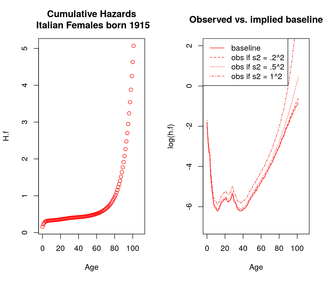
Figure 5.1: Italian Females vs Males, born 1915 \(\sigma^2=.5^2=.2^2=1^2\)
par(mfrow = c(1,2))
## title("Cumulative Hazards\n Italian Females born 1915")
foo <- my.dt[, plot(Age, log(h.f), type = "l", ylim = c(-7, 2), col = "red",
                    main = "Observed vs. implied baseline")]
foo <- my.dt[, lines(Age, log(h0.f.5), lty = 2, col = "red")]
ugh <- my.dt[, lines(Age, log(h.m), type = "l", col = "blue")]
ugh <- my.dt[, lines(Age, log(h0.m.5), lty = 2, col = "blue")]
legend("topleft", legend = c("female observed",
                             "female baseline",
                             "male observed",
                             "male baseline"),
       col = c("red","red", "blue", "blue"), lty = c(1,2, 1,2))
## now do difference
foo <- my.dt[, plot(Age, h.m/h.f, type = "l", col = "black",
                    ylab = c("h.m/h.f"),
                    main = "Male-female hazard ratio")]
foo <- my.dt[, lines(Age, h0.m.5/h0.f.5, lty = 2)]
legend("topright", legend = c("observed",
                              "implied baseline"),
##       col = c("red","blue"),
       lty = 1:2)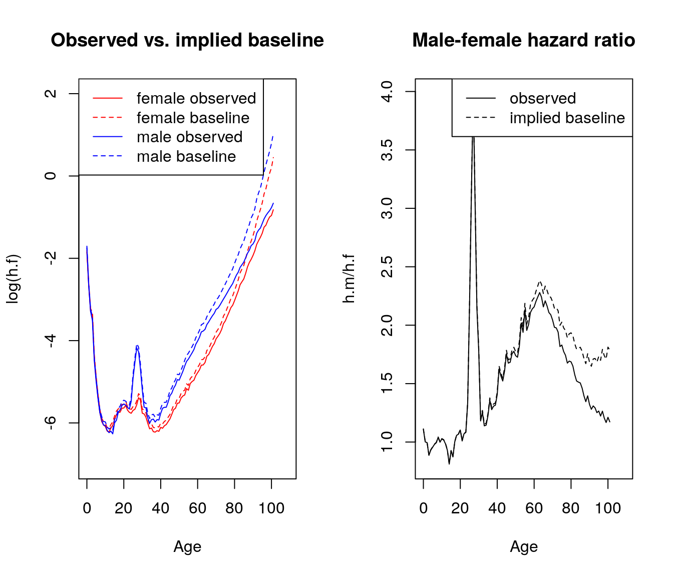
Figure 5.2: Italian Females vs Males, born 1915 \(\sigma^2=.5^2\)
Much bigger convergence in “observed” than in baseline
5.2.5 Application
German Rodriguez App for Black-White Crossover
5.3 Student Presentation
References
Coale, Ansley J, and Ellen Eliason Kisker. 1986. “Mortality Crossovers: Reality or Bad Data?” Population Studies 40 (3): 389–401.
Manton, Kenneth G, and Eric Stallard. 1981. “Methods for Evaluating the Heterogeneity of Aging Processes in Human Populations Using Vital Statistics Data: Explaining the Black/White Mortality Crossover by a Model of Mortality Selection.” Human Biology, 47–67.
Vaupel, James W, and Trifon I Missov. 2014. “Unobserved Population Heterogeneity: A Review of Formal Relationships.” Demographic Research 31: 659–86. https://www.demographic-research.org/Volumes/Vol31/22/.