Chapter 11 Demographic theory and COVID-19

11.1 Outline

• Formal demography of epidemic mortality

Additional resources:

• For more details and insights refer to Goldstein and Lee (2020)

11.2 Motivating questions

1. How does age-structure of population affect epidemic mortality?
2. How does mortality change affect life expectancy in normal times?
3. How much remaining life is lost from an epidemic?

11.3 Population aging

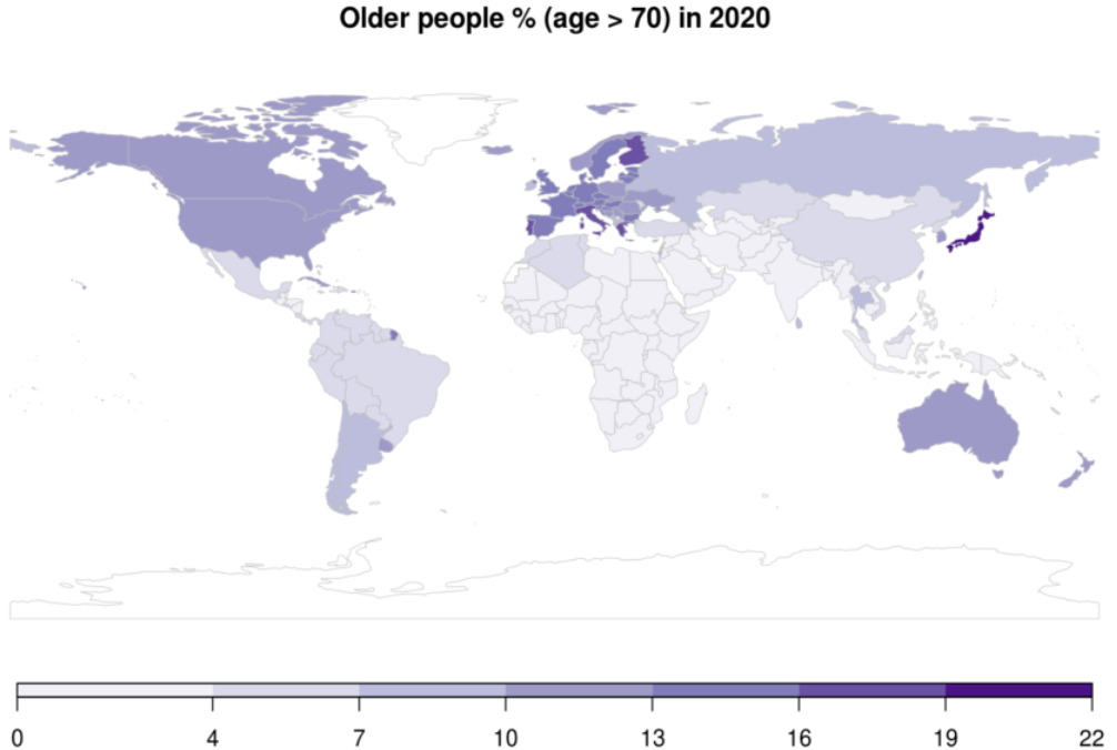
Worldwide distribution of the elderly

Source: Tuljapurkar and Zuo

• Covid19 has affected the elderly the most which accounts for a substantial share of the population of the Global North.

11.3.1 Stable theory

Let’s revist the stable population theory to understand a change the importance of population structure on epidemic dynamics. The underlying assumptions to a stable population are that i) age-specific mortality and fertility rates are fixed over a long period, ii) age-structure is constant and iii) population closed to migration.

• In this context, the population of age \(x\) in year \(t\) depends on the births (\(B(t)\)) and the survivorship: \[N(x,t)= B(t-x)\ell(x) =B(t)e^{-rx}\ell(x)\].

• The total population in year \(t\) is then \(N(t)=\int_{0}^{x} N(a,t)da = B(t)\int_{0}^{x} e^{-ra}\ell(a)da\)

• Proportion of stable population at age x: \[ c(x) = \frac{N(x,t)}{N(t)}=\frac{B(t)e^{-rx}\ell(x)}{N(t)} =b e^{-rx}\ell(x) \] where \(b\) is the birth rate \(\left(b=\frac{B(t)}{N(t)}\right)\). Note that the age-structure and the birth rate are independent of \(t\) in the notation.

• Birth rate of a stable population: As \(\int_0^{x} c(a)da =1\), \[\int_{0}^{x} b e^{-ra}\ell(a)da =1 \\ b = \frac{1}{\int_{0}^{x} e^{-ra}\ell(a)da} \] Using the Lotka-Euler equation we find that: \[ \]

• Now we look at the crude death rate (CDR), which is the share of deaths \(D(t)\) in a given population $$

  \[\begin{aligned} CDR &= \frac{D(t)}{N(t)}\\ & = \frac{\int_{0}^{x} D(a,t)da}{\int_{0}^{x} N(a,t)da} \\ & = \frac{\int_{0}^{x} h(a) N(a,t)da}{B(t)\int_{0}^{x} e^{-ra}\ell(a)da} \\ &= \frac{B(t)\int_{0}^{x} h(a) e^{-ra}\ell(a)da}{B(t)\int_{0}^{x} e^{-ra}\ell(a)da} \end{aligned}\]

  $$ where \(h(x)\) is the hazard of dying at age \(x\).

• Therefore, in a stable population with growth rate \(r\) we have a crude death rate that depends on the intrinsic growth rate: \[CDR(r) = {\int e^{-ra} \ell(a) h(a) \, da \over \int e^{-ra} \ell(a) \, da} \]

• How does the CDR vary with growth rates?
  We can change \(r=b-d\) to make the population younger or older: \(r>0 \Rightarrow\) younger population as \(b>d\) but if \(r<0 \Rightarrow\) then the population is older \[ \begin{aligned} \frac{d}{dr} \log CDR(r) &= \frac{d }{dr}\log \int e^{-ra} \ell(a) h(a) da - \frac{d}{dr}\log \int e^{-ra} \ell(a)da\\ & = -\frac{\int a e^{-ra} \ell(a) h(a) da}{\int e^{-ra} \ell(a) h(a) da} + \frac{\int a e^{-ra} \ell(a) da}{\int e^{-ra} \ell(a) da} \\ \end{aligned}\]
  If we assume a stationary population, such that \(r=0\), \[ \begin{aligned} \frac{d}{dr} \log CDR(r) & = -\frac{\int a \ell(a) h(a) da}{\int \ell(a) h(a) da} + \frac{\int a \ell(a) da}{\int \ell(a) da} \\ & =-\frac{\int a D(a) da}{\int D(a) da} + \frac{\int a \ell(a) da}{\int \ell(a) da} \\ & = -\int a D(a) da + \frac{\int a \ell(a) da}{\int \ell(a) da} \end{aligned} \] Here, \(l(x)h(x)\) is the density of deaths by age \(x\) and \(\int_0^x D(a)da =1\). This is a classic result (from Lotka) where the rate at which \(r\) changes affects the CDR through the mean age (\(A\)) and the life expectancy at birth (\(e_0\)): \[{d \log CDR(r) \over dr}|_{r = 0} = A - e(0)\]

  • An example: Let \(A=40\) and \(e_0=80\) then \({d \log CDR(r) \over dr}|_{r = 0}\approx -40\) If US and India had same age-specific mortality, but India grew 1 percent faster, what would the ratio of their crude death rates be? Both countries experience the same CDR(r) but for India \(dr=0.01\): \(d \log CDR(r) = (-40)(0.01) = -0.4\) The death rate will be 40% lower in the US relative to India conditional on age structure NOTE FOR JOSH: Not sure of interpretation of this example.

  • Now, if Covid-19 increases hazards at all ages by the same amount proportion in both countries, what will the ratio of their crude death rates be? 4 deaths in India per 10 deaths in the US.

11.4 Keyfitz’s entropy

• Assume that there is a proportional difference in mortality rates across all ages such that: \[\mu^*(x) = (1 + \Delta) \mu_0(x)\] where \(\delta \in (0,1]\).

  • The new survivoship is:

  \[ \begin{aligned} \ell^*(x) &= e^{-\int_0^{x}\mu^{*}(a)da}\\ & = e^{-(1+\Delta)\int_0^{x}\mu(a)da} \\ & =\ell(x)^{1+ \Delta} \end{aligned}\]

  • So, \(H^*(x) = (1 + \Delta) H(x)\).
  • Life expectancy at birth is:

  \[e_0^{*} (x) = \int_{0}^x \ell(a)^{1+\Delta}da\]

  • How does the new life expectancy change with the increase in mortality at al ages?

  \[ \frac{de_0^{*} (x)}{d\Delta} = \int_{0}^x (\log\ell(a))\ell(a)^{1+\Delta}da\] This quantity will never be positive, as \(\ell(a) \leq 1\) such that \(\log(\ell(a))<0\). As the \(\Delta\) factor increases, life expectancy at birth falls.

  • Entropy is defined as

  \[ {\cal H} = {d \log e_{0}(0) \over d \Delta} = {-\int \ell(x) \log \ell(x) \, dx \over e_{0}(0)} \] Reverse order of integration to get \[ {\cal H} = {\int d(x) e(x) \, dx \over e_{0}(0)} \] NOTE TO JOSH: don’t really know what the last formula is supposed to convey.

11.5 Loss of person years remaining

Before epidemic the person year remaining (PYR): \[ PYR = \int N(x) e(x) \, dx \] After (‘’instant’’) epidemic \[ PYR = \int \left[ N(x) - D^*(x) \right] e(x) \, dx \] Proportion of person years lost \[ \int D^*(x) e(x) \,dx \over \int N(x) e(x)\, dx \]

11.6 Stationary theory

If

1. \(\color{red}{\mbox {Stationarity}}\, N(x) \propto \ell(x)\)
2. \(\color{red}{\mbox {Proportional hazards}}\, M^*(x) = (1 + \Delta) M(x)\)

Then Proportional loss of person years: \[ \color{red}{ {-d \log PYR \over d \Delta} = {H \over A} = {\mbox{Life table entropy} \over \mbox{Mean age of stationary pop}}} \approx {0.15 \over 40} = 0.0038 \]

A doubling of mortality in epidemic year (\(\Delta = 1)\) causes ``only’’ a 0.38% loss of remaining life expectancy. % Average person who dies loses \(e^\dagger \approx 12\) years.

These numbers seem small, but:

• Even an epidemic doubling mortality has small effect on remaining life expectancy (\(\approx \color{red}{2 \mbox{ months}}\) per person)
  • But all-cause mortality also small (\(\approx \color{red}{2 \mbox{ months}}\) per person)
  • Covid-19: 1 million deaths \(= 30\)% more mortality, but older \ (\(\approx \color{red}{2 \mbox{ weeks}}\) per person)

Barbi, Elisabetta, Francesco Lagona, Marco Marsili, James W Vaupel, and Kenneth W Wachter. 2018. “The Plateau of Human Mortality: Demography of Longevity Pioneers.” Science 360 (6396): 1459–61.

Batini, Chiara, Pille Hallast, Åshild J Vågene, Daniel Zadik, Heidi A Eriksen, Horolma Pamjav, Antti Sajantila, Jon H Wetton, and Mark A Jobling. 2017. “Population Resequencing of European Mitochondrial Genomes Highlights Sex-Bias in Bronze Age Demographic Expansions.” Scientific Reports 7 (1): 1–8.

Bongaarts, John, and Griffith Feeney. 1998. “On the Quantum and Tempo of Fertility.” Population and Development Review, 271–91.

Burkimsher, Marion. 2017. “Evolution of the Shape of the Fertility Curve: Why Might Some Countries Develop a Bimodal Curve?” Demographic Research 37: 295–324.

Coale, Ansley J, and Ellen Eliason Kisker. 1986. “Mortality Crossovers: Reality or Bad Data?” Population Studies 40 (3): 389–401.

Felsenstein, Joseph. 2005. “Theoretical Evolutionary Genetics Joseph Felsenstein.” University of Washington, Seattle. https://evolution.gs.washington.edu/gs562/2017/pgbook.pdf.

Goldstein, Joshua R, and Ronald D Lee. 2020. “Demographic Perspectives on Mortality of Covid-19 and Other Epidemics.” National Bureau of Economic Research.

Hahn, Matthew W, and R Alexander Bentley. 2003. “Drift as a Mechanism for Cultural Change: An Example from Baby Names.” Proceedings of the Royal Society of London. Series B: Biological Sciences 270 (suppl_1): S120–S123.

Harris, Theodore Edward. 1964. “The Theory of Branching Process.” https://www.rand.org/content/dam/rand/pubs/reports/ 2009/R381.pdf.

Hastie, Trevor, Robert Tibshirani, and Jerome Friedman. 2009. The Elements of Statistical Learning: Data Mining, Inference, and Prediction. Springer Science & Business Media.

Horiuchi, Shiro. 2003. “Interspecies Differences in the Life Span Distribution: Humans Versus Invertebrates.” Population and Development Review 29: 127–51.

“Introduction to Probability.” 2006. https://math.dartmouth.edu/~prob/prob/prob.pdf.

Manton, Kenneth G, and Eric Stallard. 1981. “Methods for Evaluating the Heterogeneity of Aging Processes in Human Populations Using Vital Statistics Data: Explaining the Black/White Mortality Crossover by a Model of Mortality Selection.” Human Biology, 47–67.

Rodriguez, Germán. 2001. “Unobserved Heterogeneity.” https://data.princeton.edu/pop509/UnobservedHeterogeneity.pdf.

Steinsaltz, David R, and Kenneth W Wachter. 2006. “Understanding Mortality Rate Deceleration and Heterogeneity.” Mathematical Population Studies 13 (1): 19–37.

Sullivan, Rachel. 2005. “The Age Pattern of First-Birth Rates Among Us Women: The Bimodal 1990s.” Demography 42 (2): 259–73.

Vaupel, James W, Kenneth G Manton, and Eric Stallard. 1979. “The Impact of Heterogeneity in Individual Frailty on the Dynamics of Mortality.” Demography 16 (3): 439–54.

Vaupel, James W, and Trifon I Missov. 2014. “Unobserved Population Heterogeneity: A Review of Formal Relationships.” Demographic Research 31: 659–86. https://www.demographic-research.org/Volumes/Vol31/22/.

Wachter, Kenneth W. 2014. Essential Demographic Methods. Harvard University Press.

Waldron, Hilary. 2007. “Trends in Mortality Differentials and Life Expectancy for Male Social Security-Covered Workers, by Socioeconomic Status.” Soc. Sec. Bull. 67: 1.

References

Goldstein, Joshua R, and Ronald D Lee. 2020. “Demographic Perspectives on Mortality of Covid-19 and Other Epidemics.” National Bureau of Economic Research.